-
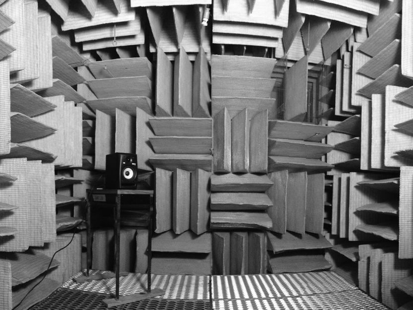 Acoustics
Acoustics engineers perform research on problems of both a basic and applied nature in physical...
Learn more
-
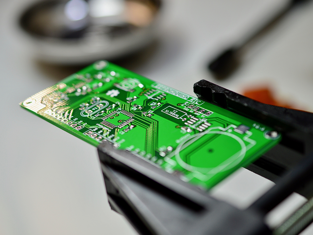
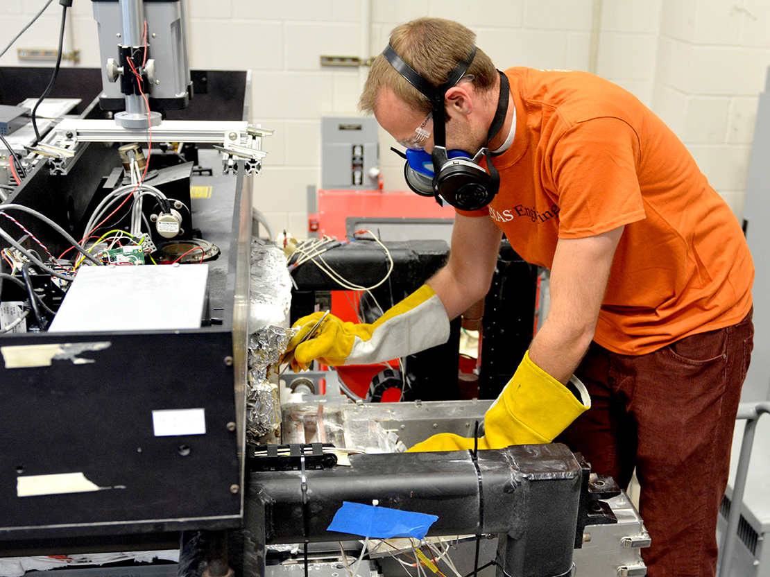 Advanced Manufacturing and Design
Advanced Manufacturing and Design uses technological advances to create products and systems that...
Learn more
-
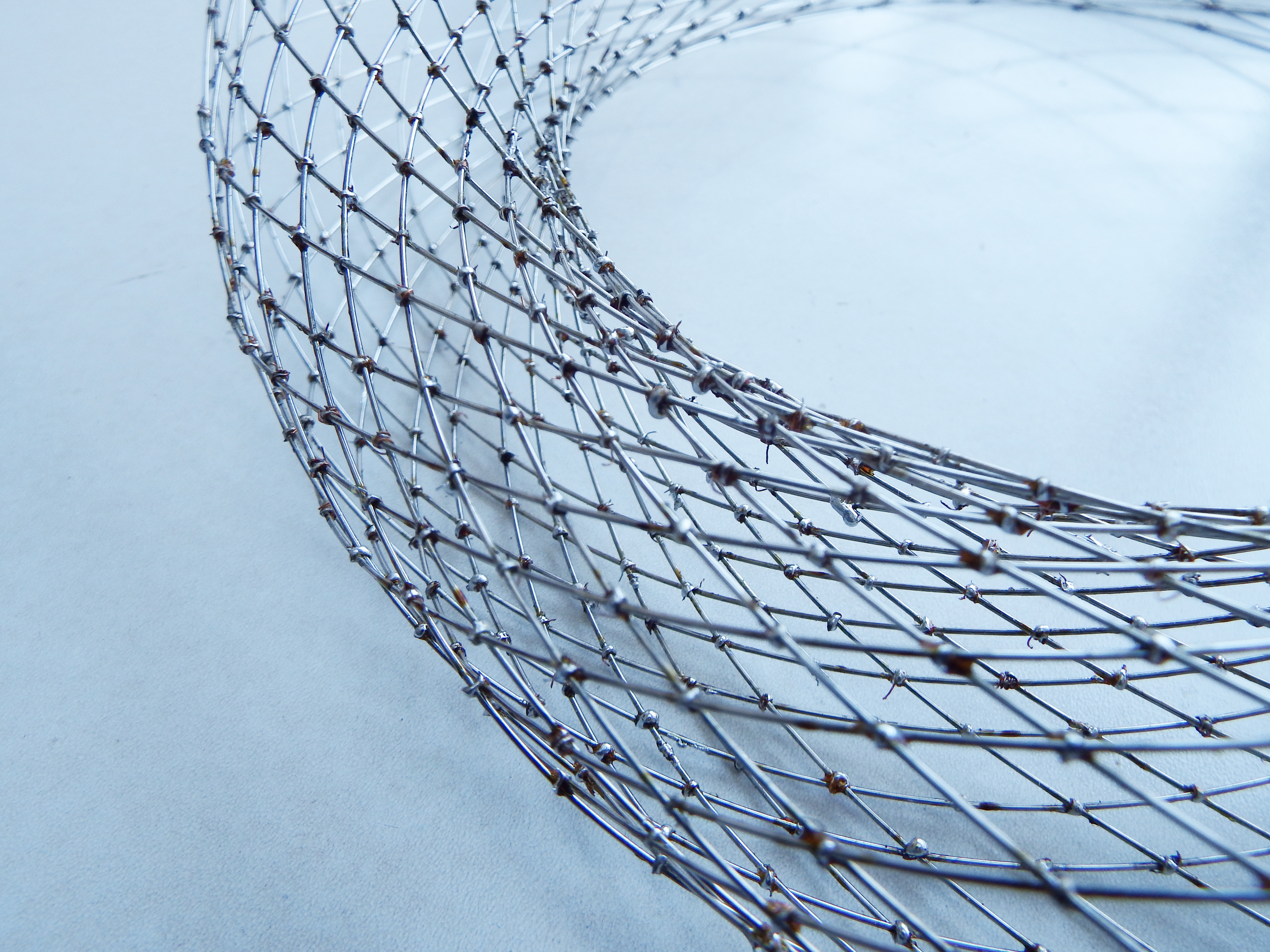
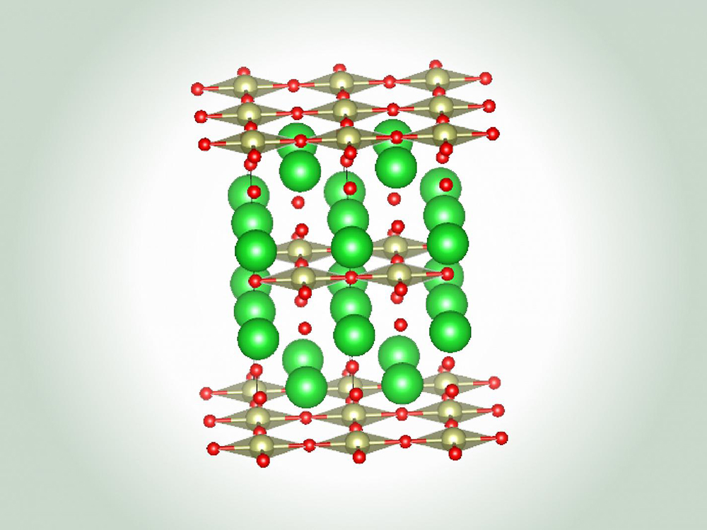 Advanced Materials Science and Engineering
The Advanced Materials Science and Engineering research area in the Walker Department of...
Learn more
-
 Analytics and Probabilistic Modeling
Decisions are often difficult because the outcome is uncertain. Researchers focused on Analytics...
Learn more
-
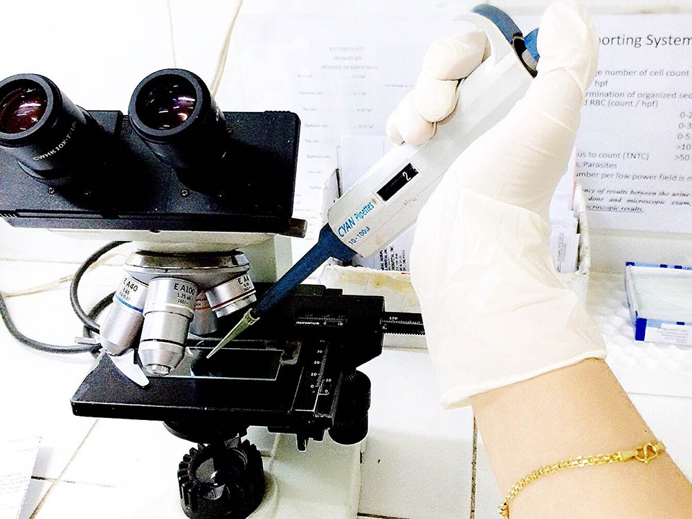 Biomechanical and Biomedicine
Biomechanics is the application of fundamental mechanical engineering principles to biological...
Learn more
-
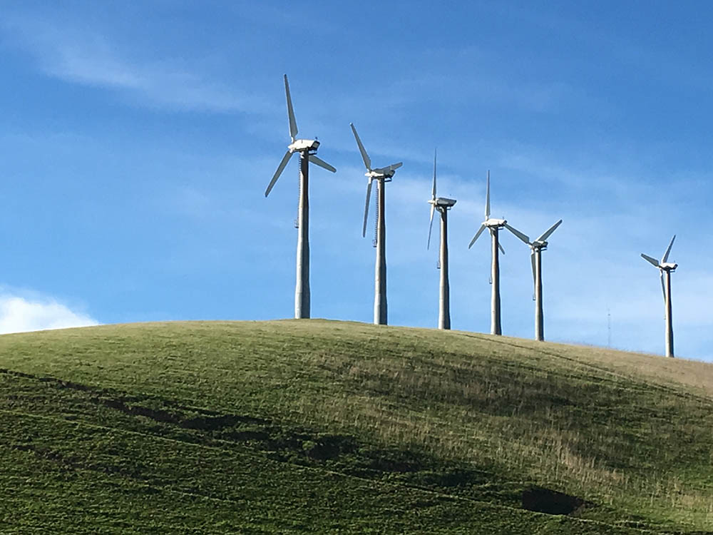 Clean Energy Technology
Clean energy technology research focuses on advancing clean energy technology at every stage, from...
Learn more
-
 Complex Systems
Complex Systems includes the science, mathematics and engineering of systems with simple...
Learn more
-
 Computational Engineering
Computational engineers develop and apply the computational models, data assimilation techniques,...
Learn more
-
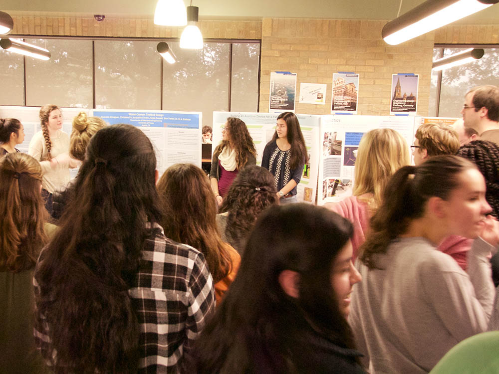 Engineering Education
Engineering Education research focuses on understanding how best to recruit, retain and prepare a...
Learn more
-
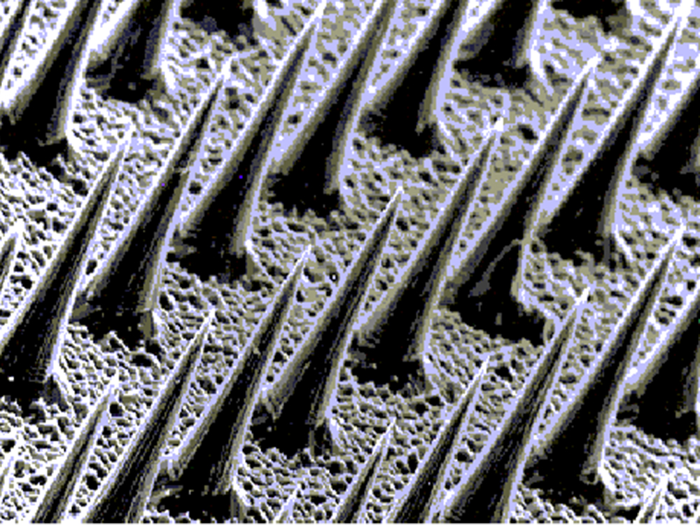 Nano and Micro-scale Engineering
As materials, mechanisms, and machines are scaled down to the micro- and nano-scales, new physical...
Learn more
-
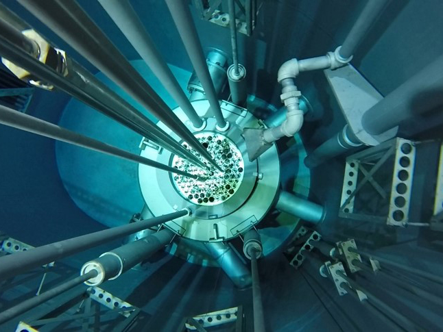 Nuclear and Radiation Engineering
Encompasses health physics, radiation engineering, research reactor beam port experiments,...
Learn more
-
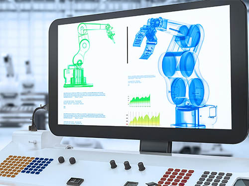
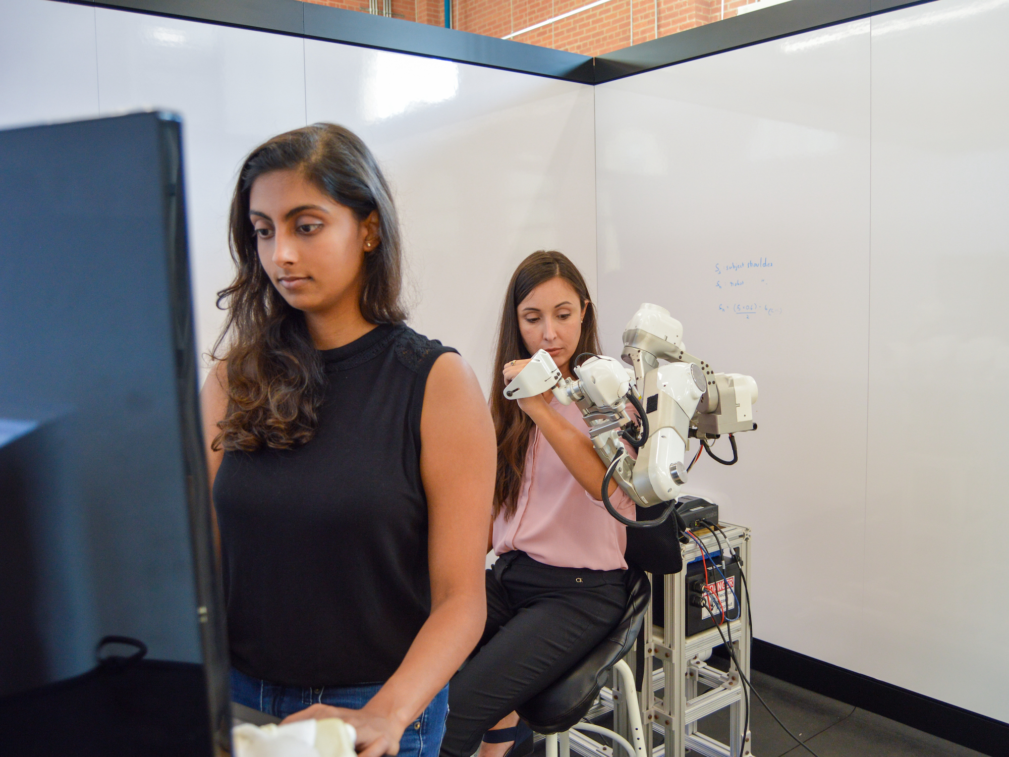 Robotics and Intelligent Mechanical Systems
Robotics and intelligent machines are emerging as prime technologies that can provide a wide range of...
Learn more